Editor’s Note: This is the second of a series of tips and tricks in Excel that will help any and every PPC Advertiser. You can read the first part here.
Microsoft Excel is an extremely powerful and versatile resource for PPC Advertising. It is used in a number of ways, whether it’s prepping ads to bulk upload into Google Ads Editor or doing a deep dive analysis into your account’s performance. Having the ability to download data into a .csv file directly from Google and Microsoft Ads UI, combined with the intricate data filters they offer, allows you to create some extremely valuable and insightful custom reports.
The amount of data is usually why you use Excel for PPC purposes, instead of just using the data within the UI or the reporting tab of Google or Microsoft. So staying organized will definitely help you finish whatever PPC task you’re working on much more efficiently.
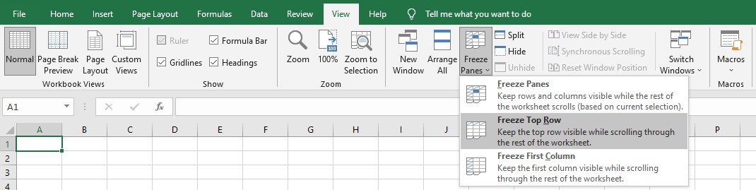
The one thing I do pretty much every single time I create a spreadsheet is to freeze the top row, so it never leaves your screen. That top row acts as your header. Because again, when downloading custom reports from Google Ads or Microsoft Ads, the volume of data is typically big enough that you’re going to want to freeze that top row. Otherwise, you’ll constantly be scrolling up and down, trying to figure out what number means what. You can find the option to freeze rows in the “Window” section of the “View” tab shown below.

Also, it can be very helpful to freeze that first column as well. Typically the first column will be something along the lines of a search term, keyword, product, campaign, or ad group. So being able to easily attribute that data back to the correct item is pretty important.
Another thing that is a staple of any spreadsheet I work on is using filters. Adding in filters to your headers enables you to really dissect and get into the weeds of the data you’re looking at. Filters allow you to sort your columns however you like. You can sort by most spend to least spend or most conversions to least conversions. And you may also, of course, filter columns. Filters also give you the ability to temporarily exclude items that are irrelevant for your data analysis or to filter ONLY the data you want to see.
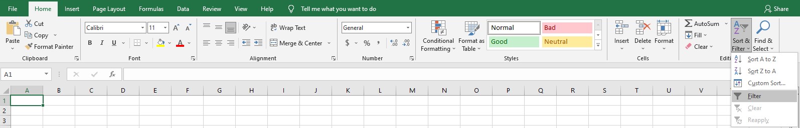
For example, say you’re looking at a keyword performance report for the last 30 days. You are able to use filters to hide any keyword that has zero conversions, $0 in spend, or zero clicks. Or you can filter out anything below $50 in spend. There are a plethora of options when it comes to filtering your data. The filter option can be found in the “Editing” section of the “Home” tab shown below.
So now that you have your headers locked into place, you’re ready to start filtering your little heart out.
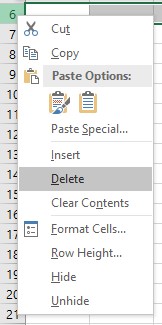
First off, every downloaded report will have some unnecessary rows at the top of the sheet. These rows typically include the type of report it is and the time frame for the report. I like to delete them and instead use the sheet tab at the bottom of the screen to display that information. You can do this by right-clicking on the number of the row on the far left of your screen. This selects the entire row, and then you’ll see options to either hide the row or delete the row entirely.
Then, I’ll go ahead and remove any redundant columns that Google or Microsoft will add to your report. The content of these columns varies depending on what kind of report you’re looking at, whether it’s a campaign, keyword, product report, or if the report came from Google or Microsoft. Generally, this is a user-preference kind of thing, but there will typically be columns for currency, status, budget, bid, etc. Most of these columns are redundant when taking a deeper look into custom reports.
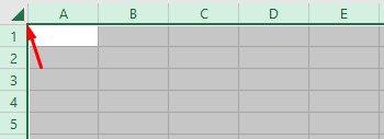
Finally, I’ll put the finishing touches on the spreadsheet by cleaning up some of the cosmetics. This might seem silly but can really make an impact if you’re preparing a report for a client. Again, when using Excel for PPC purposes, you’re dealing with such a large volume of data that it can be overwhelming to look at. So anything you can do to either break it down or clean it up into a more digestible piece of information can be helpful. One way of doing so is to make sure the sizing of the columns is all appropriate. You can do this by clicking the green arrow in the top right of your screen where the rows and columns meet. Clicking that selects the entire spreadsheet.
Then you simply double-click the margin in between two columns, and the spreadsheet will automatically resize all columns and rows to exactly fit the text or data in it.
After you have done all of this, your spreadsheets should look sharp. You are now ready to dive in and start making some well-informed decisions to help drive paid search performance.